
See the shape
of your source code
Code Contour measures a codebase and shows you what it is made of. Point it at a folder and it reads every file, in 81 languages, and reports lines, comments, methods, cyclomatic and cognitive complexity, Halstead volume and maintainability, file by file and method by method. Charts turn those numbers into something you can act on, a click on any of them selects the files behind it, and the whole run exports as CSV, HTML, JSON or a printed PDF report.
Numbers you can act on
Code Contour is a metrics tool for people who have to look after a codebase they did not write all of. It measures what is there, says how sure it is, and never hides a file it could not read.
Every number has a source
Complexity is McCabe, cognitive complexity is Campbell, the maintainability index is the Microsoft form. Nothing here is invented, and this guide says exactly how each number is arrived at, so you can check it against your own reading of the code.
Charts you can click
Every chart is drawn from the rows on screen, and a click on a bar, a spoke, a slice or a rectangle selects the files behind it. A picture nobody can act on is a screensaver.
Honest about itself
A file that could not be read is listed with the reason. A language it is not sure about carries a confidence. Code that is not yours, generated or vendored, is marked rather than quietly counted.
Private and offline
Your source never leaves your PC. No cloud, no telemetry, no account. The project file and every export are written where you put them.
Native and fast
A compiled Windows application with no runtime to install. It reads files that other programs are still writing, and it never blocks on a lock.
A history, not a snapshot
Keep an analysis in the project and it becomes a point you can come back to. A trend shows where the codebase went, and a work report says what was written between any two points.
Where the idea came from. Code Contour was inspired by Source Monitor, a tool many developers remember and which is now frozen legacy. Aelyo Softworks is not affiliated with it in any way, has no relation to its authors or its owners, and none of its open source version was used or looked at in the making of this product. Code Contour is not a clone of it. It is a new application, written from nothing, with its own analysis engine, its own metrics, its own charts, its own reports, its own command line and its own file format, and with features that tool never had. What the two have in common is the belief that a codebase is worth measuring.
Installation
Code Contour is a single, self-contained Windows application. Once installed it appears in your Start menu and registers the .codecontour project type.
Get Code Contour
Code Contour is distributed through the Microsoft Store, so it stays up to date automatically and installs cleanly with no extra runtimes.
⬇ Get it from the Microsoft StoreNothing to configure. Code Contour opens on an empty project. Add a folder, press F5, and you have your first analysis. Double-clicking a .codecontour file in Explorer opens that project.
The Window
One window holds everything. A panel down the left says what is being measured, the table in the middle is the result, and a summary along the bottom totals whatever the table is showing.
Folders
The folders this project covers. Add, remove, or change one, and drop folders straight onto the window.
Analyses
The runs this project has kept, most recent first, with the current run at the top when it has not been kept yet. Keep, remove, show and compare from here.
The table
One row per file. Sort by any column, right click a header to choose which ones show, right click a row for everything you can do to that file.
The aggregate line
Under the table, the totals of the rows on screen. It follows every filter, so it always describes what you are looking at rather than what was measured.
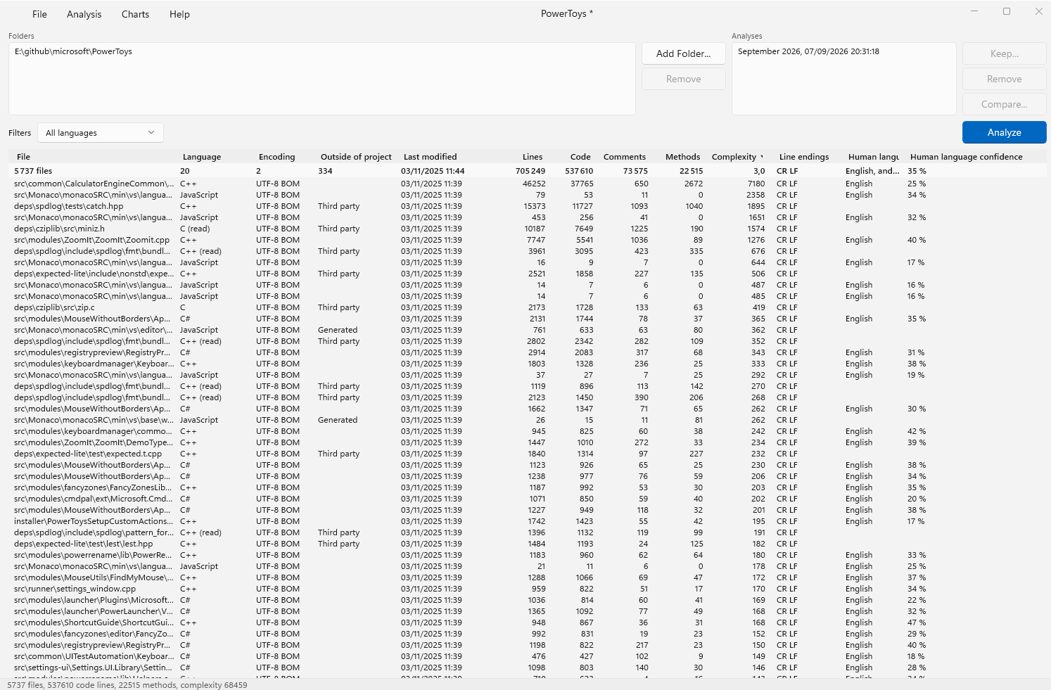
The pictures in this guide were taken of Microsoft's PowerToys repository, which is open source under the MIT licence. It is 5 737 files in 20 languages, which is a fair likeness of the kind of codebase this tool is for.
The summary answers each column in its own way. A count is totalled, a complexity is averaged, an encoding says how many distinct ones there are, and the human language column says which languages were found and how sure it was.
Projects & Folders
A project is a name, a .codecontour file, and the folders it covers, together with the rules it was measured under and the analyses it has kept.
Adding folders
Use Add Folder... in the Folders panel, the same entry at the top of the Analysis menu, or drop a folder onto the window. A project can cover as many folders as you like, in as many languages as you like. Sub-folders are walked automatically.
The walk goes past the folders the system hides, a tool's cache, a recycle bin, a volume's own bookkeeping. That is a project setting and it is on by default. A folder you asked for by name is never judged that way, so a project whose root is hidden is scanned anyway.
Saving
File → Save Project writes the .codecontour document, which holds the folders, the rules, and every analysis kept. It is compressed JSON, so a project with a long history stays small. Recent projects are listed under File → Recent Projects, with entries to clear the list and to drop the projects whose file is gone.
The counting rules belong to the project and are frozen once its first analysis is kept. A trend measured under two different sets of rules would move for a reason that is not the code, so Code Contour refuses to change them rather than let that happen.
Running an Analysis
Analysis → Analyze, or F5, measures every file under every folder of the project. The status line says what it is doing, and you can stop it at any point.
While it runs
A run is not one long wait, so the line says which of four things it is in, getting ready, reading what the repositories say about their own files, looking for files, and measuring them. Only the last can be counted against a total, and the walk names the folder it is in as it goes.
Stopping keeps what was measured so far and says so. Nothing is lost, and running it again is all it takes to have the whole thing.
Second checkouts of the same code
A git worktree is a second checkout of a repository you already have, and they have become common: an AI agent is given one to work in, or you keep one to build the previous release while you edit the next. Under a folder being measured, one of those is the project's own files a second time, and counting them twice says the codebase doubled overnight and every file of it has a twin.
So a worktree found under a folder of the project is walked past, and the run says so: a clause on the status line, a line in the header of every report, and Analysis → Second checkouts passed over, which lists each one with the repository it is a checkout of, beside the list of files that could not be read. It is the one skip worth a sentence of its own, because bin and node_modules hold nothing of yours while this holds all of it again, and every folder a run passed over is listed under Analysis → Folders left out. The churn of two worktrees of one repository is read once rather than added to itself. A submodule is not a worktree and stays: it is code of its own that happens to live inside another repository. And a worktree you name as a project folder yourself is measured like any other folder, since asking for one on purpose is a different thing from meeting one on the way.
Files another program is holding
Every file is opened read only and shared as widely as a reader can share it, so a log or a database journal is read while its owner goes on writing it. Nothing waits for a lock and nothing retries, because a scan of a live tree would never end if it did.
A file whose owner shares nothing at all is counted out of the run, and never silently. The summary says how many there were, and Analysis → Files that could not be read lists them with the reason the system gave.
Encodings and line endings
Every file's encoding is detected as it is read, from its byte order mark where it has one and from its content where it has none, and the analysis reports which encoding each file turned out to be. A project says which encoding to assume for a file with no mark, and any encoding Windows knows can be chosen, 116 of them.
Line endings are reported the same way, and the summary says how many files disagree with the rest. A codebase where thirty files out of five thousand end their lines differently is a codebase with an editor setting somebody has not shared, and it is the kind of thing nobody notices until a diff is unreadable.
The first analysis of a project also decides what the project thinks is normal. Later runs are measured against the same bands, which is what makes the Kiviat chart worth reading.
Languages
Code Contour reads 81 languages, from C and C++ to Rust, Go, Swift, Kotlin, Zig, COBOL and Fortran, plus markup and data formats that a repository is full of and that no metrics tool should pretend are code.
Code, markup, data
Every language is one of three kinds, and the kind decides what is measured and what is merely counted:
Code
Measured in full, methods, complexity, block depth, calls and maintainability. This is what the metrics are about.
Markup
HTML, XML, CSS, Markdown. Lines and comments are real, control flow is not, so nothing pretends there is any.
Data
JSON, TOML, INI, Makefiles, Dockerfiles, protobuf. Counted, and JSON is genuinely measured, since it is half of what a modern repository holds.
Whether markup and data files are looked at is a project setting, so a project can be about its code alone.
The whole list
Every language Code Contour reads. The dot says which kind it is: code in blue, markup in green, data in dark blue.
How each one is measured
Most languages are measured routine by routine. Code Contour finds the methods, functions or procedures, gives each its own complexity, statements, block depth and calls, and rolls them up to the file. That is the grain the metrics were designed for.
A few languages have no routine a lexer can honestly find, and those are measured as the whole they are written as, one set of numbers for the file rather than one per routine. COBOL is the clearest case: a paragraph is a name followed by a full stop and cannot be told apart from a sentence, and a section of the data division is not a routine at all. Prolog is the same, a clause is not a procedure. Nothing is invented for them, and their files simply carry no method count.
Only real code is measured. A file that is code first and markup second, a .razor, a .vue, a .svelte, is code here, since that is what somebody writing it is doing. A file that is markup with code sprinkled in is markup.
What JSON's numbers mean. JSON is measured rather than merely counted, since it is half of what a modern repository holds, but it has no control flow and nothing here pretends otherwise. A member is a statement. An object or array is a block, so depth is the nesting a reader has to follow. Complexity is that deepest nesting rather than a count of paths, because there are no paths. Anything whose extension ends in json is treated as JSON, since the format spawns dialects faster than any table can name them.
Extensions
A file's extension decides its language, and you can override any of it. File → File Extensions lists every extension Code Contour has an opinion about, what was decided for it, and lets you say otherwise, including saying that files of that kind hold no code at all. The mapping belongs to you rather than to one project, so it follows you from project to project.
An extension met for the first time is reported rather than guessed at, so a codebase full of an extension nobody has taught it about does not silently read as nothing.
The language it is written in
Separately from the programming language, Code Contour can tell you what human language the comments and strings are written in, with a confidence for each answer. Windows detects it, so it costs no dependency and no network. On a codebase worked on by several teams this is often the most surprising column in the table.
Metrics
Every number has a source, and none of them is this tool's invention.
| Lines | Every line of the file, blank ones included. |
| Code lines | Lines that carry code. Blank lines and comment lines can each be counted out, per project. |
| Comments | Comment lines, with documentation comments countable separately. |
| Statements | What the language ends with a separator, per method and per file. |
| Methods | Functions, methods, procedures, whatever the language calls them. |
| Cyclomatic complexity | McCabe. One, plus one for each if, for, foreach, while, case, catch, &&, || and ?. An else and a default add nothing, since they open no path that was not already counted. |
| Cognitive complexity | Campbell. A whole switch costs one however many labels it has, an else costs one and nests nothing, a run of the same boolean operator costs one, and anything nested costs one more per level. It measures how hard code is to follow rather than how many paths it has. |
| Block depth | How deeply the code nests, per method and at its worst in the file. |
| Calls | How many calls a method makes. |
| Halstead volume | N log₂ n over the token stream. |
| Maintainability index | The Microsoft form, computed per method, which is the grain it was designed for, and averaged over a file by lines. A file with no method at all falls back to its own tokens. |
| Percent branches | Decision points over statements. |
| Percent comments | Comment lines over all lines. |
Cyclomatic complexity, in detail
McCabe's measure counts the paths through a routine. Start at 1, the one path taken when nothing branches, then add 1 for every point where the code can go two ways:
if, elif, a ternary ?for, foreach, while, docasecatch&&, ||An else and a default add nothing. They open no path that the if or the switch above them had not already opened, so counting them would count the same fork twice. A routine of 1 has one way through it. A routine of 30 has thirty, which is also, roughly, the number of tests it takes to cover.
Counting every case separately is the default. Modified complexity, a project option, counts a whole switch as one instead, on the argument that a reader takes in a table of ten labels more easily than ten separate ifs. Both are defensible, and a project settles on one before its first analysis so that its history is comparable.
Cognitive complexity, in detail
Campbell's measure asks a different question: not how many paths there are, but how hard the code is to follow. It is deliberately not the same number, and where the two disagree the disagreement is the point.
switchelseSo a && b && c costs 1, because it is one idea, while a && b || c costs 2, because the reader has to change gear in the middle. A switch over ten cases costs 1 where cyclomatic complexity charges 10, and a loop inside a condition inside a loop costs 1 + 2 + 3 where cyclomatic complexity charges 1 + 1 + 1.
Code Contour measures what a lexer can honestly see, and claims nothing more. Recursion and jumps to labels, which the original measure also charges for, add nothing here, because knowing that a call is recursive means resolving names across files and that is not what this tool does.
The language table is what tells the two measures apart, which is why a language whose case is written the other way round, Ruby's case being the head and its when the label, is still counted correctly.
Where these come from
Every measure here is somebody's published work, not this tool's idea of one:
| Cyclomatic complexity | Thomas J. McCabe, A Complexity Measure, IEEE Transactions on Software Engineering, vol. SE-2, no. 4, December 1976, pages 308 to 320. doi:10.1109/TSE.1976.233837 |
| Cognitive complexity | G. Ann Campbell, Cognitive Complexity: a new way of measuring understandability, SonarSource white paper. sonarsource.com |
| Halstead volume | Maurice H. Halstead, Elements of Software Science, Elsevier North-Holland, 1977. |
| Maintainability index | Paul Oman and Jack Hagemeister, 1992, in the form Microsoft uses in Visual Studio. learn.microsoft.com |
The maintainability index is computed exactly as that form states, per method, then averaged over a file by lines:
MI = max(0, (171 − 5.2 × ln(V) − 0.23 × CC − 16.2 × ln(LOC)) × 100 / 171)
where V is the Halstead volume, CC the cyclomatic complexity and LOC the lines of code. It lands between 0 and 100, and higher is better. A method is the grain that formula was designed for, which is why a file's figure is an average of its methods rather than the formula applied to the whole file. A file with no method at all falls back to its own tokens.
Where we knowingly differ. Percent branches here is decision points over statements. Some tools count branch statements instead, with else, break and return in the list. The two land in the same range on real code, but they are not the same number, and a figure compared across tools should be read with that in mind.
Rules you can change
A project decides how it counts, in Analysis → Project Settings, and the choices are settled before its first analysis and frozen with it:
switch counts as oneTwo more sit in the same dialog and change nothing that was measured: whether files outside the project are left out of the analysis, and whether reports carry what the repository was written. Both can be changed at any time.
Every analysis kept writes its rules down, and a report names them whenever they are not the defaults.
What counts as normal. Settings → What counts as normal holds the band each metric is compared against. That is what the Kiviat chart draws, and what makes a file "outside the band" in a report. The defaults are sensible, and a codebase with its own standards can move them.
Columns
The table shows one row per file. Choose the visible columns from Analysis → Columns or by right clicking the headers, and sort by any of them.
| File | The path, shortened in the middle when it has to give, so the name is never the part that goes. |
| Language | The programming language, with a certainty when it was not simply the extension. |
| Human language | What the comments and strings are written in, with a confidence. |
| Lines, Code, Comments | The counts. |
| Methods, Complexity | How many, and how complex the worst of them is. |
| Outside of project | Whether this file is your work, see Setting Files Aside. |
| Encoding, Line endings | How the file is written, and whether it agrees with its neighbours. |
| Size, Last modified | What the file system says. |
The aggregate line under the table follows the columns you show and the rows you have narrowed to, so it always totals what you are actually looking at.
Widths
Every column can be made wider or narrower, the file name included. A line runs down each column boundary, through the heading and the totals under it, and dragging that line moves the edge. The widths are yours and are remembered, so the table opens the way you left it, and only the columns you actually moved are stored: one you never touched still follows whatever a later version thinks is sensible.
The same three are on the menu the headers offer when you right click them, under the list of columns to show, together with Reset the column widths, which puts every column back to the width it ships with. Fitting measures the heading, the total and the rows on screen, so it fits what you can see rather than laying out every file in the project to ask.
The file name column keeps whatever room the others leave, and never gives up more than a readable minimum. Turn on enough columns and the table becomes wider than the window, at which point a scroll bar appears under it and the headings, the totals and the rows all slide together. Shift with the wheel scrolls sideways as well. The list keeps its own scroll bar against the right edge of the window, where it always was.
Filters & Selection
Narrowing the table narrows everything. Every chart draws the rows on screen, the summary totals them, and an export writes them.
The button reads Everything until you narrow something, and it means everything: every language, the code that is not your own work, and the files you set aside. Narrow it and the button says what is left, in the same words every chart and export uses to say what it covers.
By language
Show one language, several, all, or none. A codebase of half a million lines of generated data becomes readable the moment the data leaves the table.
By chart
Every chart selects. Click a spoke of the Kiviat and you get the files outside its band. Click a bar of the histogram and you get the files holding a method in that range. Sweep a rectangle over the scatter and you get the files inside it. Click a slice of the languages pie and you get that language.
Answering a chart replaces the previous answer rather than narrowing what was already narrow, so you can never paint yourself into a corner. A link above the table takes the narrowing back and shows everything again.
The selection is one thing shared by the table, the summary, the charts and the exports. Whatever you narrowed to is what an export writes, and a report says in words which rows it covers, so a file exported a month ago can still be trusted to say what it is.
Setting Files Aside
Not everything under a folder is your work, and counting it all is how a codebase comes to believe it has a million lines. Code Contour separates the two in three ways.
Outside of the project
Code that is not the project's own work is detected and marked in its own column: third party code sitting in the tree, generated files, and data scripts. Your own rule wins over the detection, so a folder you say is yours is yours. A row menu says what a file is, inside, outside, or whatever the analysis finds, and the answer is remembered for the next run.
Marked files stay in the table and stay countable. They are labelled rather than hidden, so the totals are honest and you can filter them out when you want to see only what your team wrote.
A project can go further and leave them out of the analysis altogether, Leave files outside the project out of the analysis in Analysis → Project Settings, changeable at any time since it changes nothing that was already measured. If that is how you always work, Settings → Projects has New projects leave outside code out of the analysis, and every project you make from then on starts that way. It is off to begin with: a file counted and labelled can still be filtered out of a chart, and one never measured cannot be brought back without measuring again.
Folders never measured
A folder named bin, obj, node_modules, packages, vendor or one of two dozen others is never walked into, wherever it sits. Analysis → Excluded folder names lists every one of them: turn one off to measure it, a project whose source lives in out for instance, or add your own, Generated or ThirdParty. They are names rather than paths, so one entry covers every project of a solution.
And after a run, Analysis → Folders left out says exactly which folders were passed over and why, a name, a folder Windows hides, or a second checkout. It is the answer to "where are my files", and it means no tree ever leaves an analysis without a word. The folders you set aside are in that list too, under a reason of their own, since that is where you would look for them, but they are not skipped: their files are measured and marked, which is why they are still in the table.
Exclusions
Right click a row to exclude a file, a whole folder, or every file of that extension. One click sets a branch aside and the next click gives it back. Clear all exclusions drops them all at once, after a confirmation.
What the repository says about itself
Rather than guess from a file name or a banner, Code Contour reads the rules the repository already keeps, its .gitignore and its .gitattributes. Those files are maintained by the people working there, which makes them worth more than anything a tool can infer:
linguist-generated, linguist-documentationlinguist-vendoredGit's own glob is implemented rather than approximated, so a rule behaves here exactly as it behaves for git: * stops at a slash and ** does not, a rule holding a slash is measured from the folder it was written in, a trailing slash means a folder and everything under it, and ! takes back what an earlier rule said, the last matching rule deciding. The files at and under the scanned folder are read, and the ones above it up to the repository root.
It is on by default and settled before the first analysis. Once an analysis has been kept the choice is frozen, because the analyses already kept were measured under those rules and measuring the next one differently would compare two different projects.
The Source Viewer
Double click a row, or use View in its menu, to read the file itself. It is a read-only viewer with syntax colouring, and it is where a number stops being a number.
No IDE is needed to use Code Contour, and none has to be installed to read what it measured. The viewer knows the language from the analysis, so a file is coloured the way its language should be. It opens at the line you came from when you arrived from a chart or a report link, and it moves to the next or previous row of the table without going back to it. Esc closes it.
It also keeps your place. The line you left a file at is remembered with the project, so opening it again puts you back where you were rather than at the top, which matters on the kind of file that made you open the viewer in the first place. Turn it off in Settings under Remember where you were reading in each file.
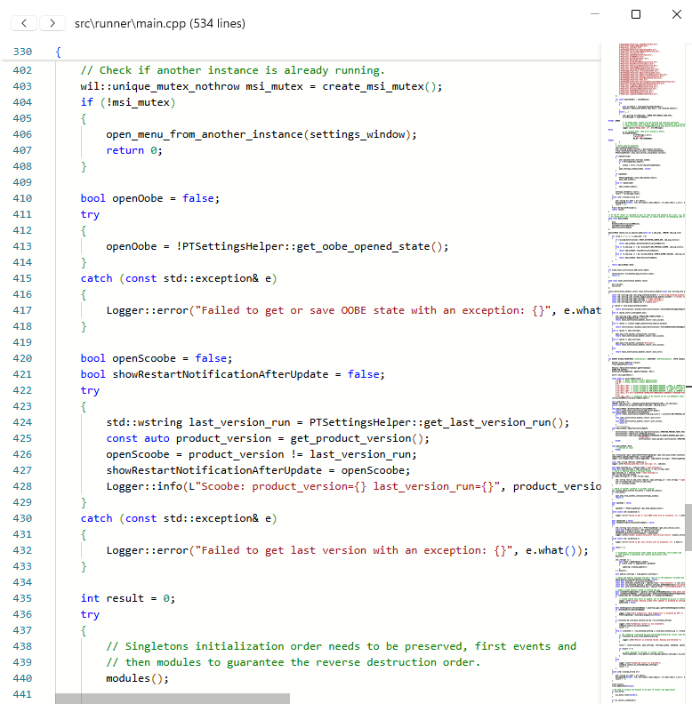
Nothing in Code Contour edits your source. The viewer opens files read only and shares them with whatever else has them open, so reading a file here never gets in the way of your editor.
Kiviat
Charts → Kiviat chart draws the rows on screen against what this project considers normal. It is the fastest way to see the shape of a codebase, and the one picture worth opening first.
Each spoke is a metric, and the band around the middle is the range that metric usually falls in. A shape that sits inside the band everywhere is ordinary code. A spoke that pushes out is where this codebase is unusual, and clicking that spoke selects the files that put it there, worst first.
A row menu also draws the Kiviat of a single file, which is the same picture asked about one thing instead of a set.
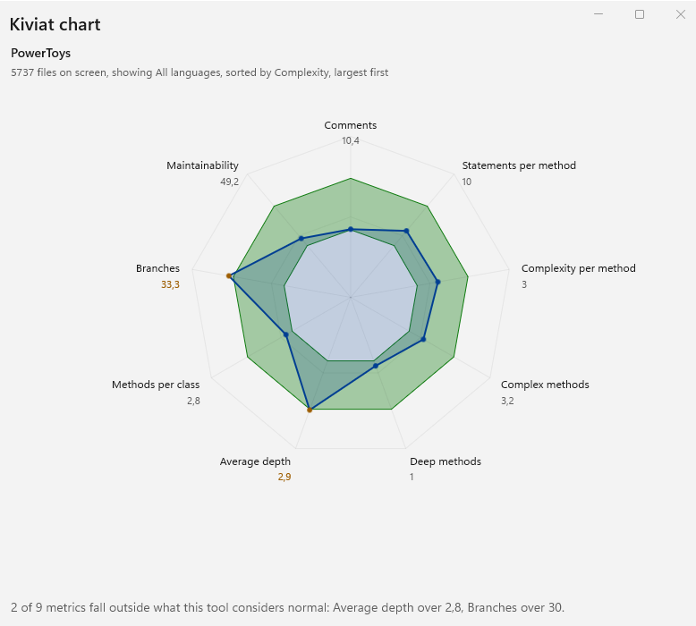
The bands come from Settings → What counts as normal. If your codebase has standards of its own, move them there and the chart starts answering your question rather than a generic one.
Map of the Code
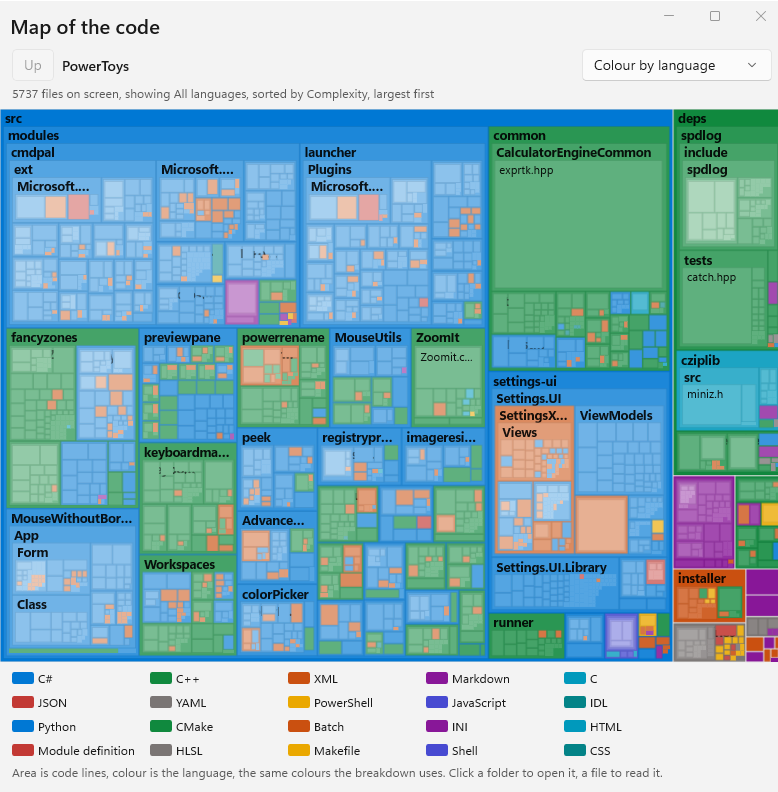
Charts → Map of the code draws every file as a rectangle, sized by its lines and nested inside its folders, so a whole codebase fits on one screen with its shape intact.
Ask it a question
The colour of the map answers one question at a time, and you choose which:
Moving around
A click on a folder opens it and the map redraws inside it. Backspace goes back up, Esc closes the map. A click on a file reads it over the map rather than instead of it, so you can look at the code and keep your place.
The map follows the table like every other chart, so filtering to one language maps that language alone.
Complexity Charts
Two charts ask about complexity, one about how it is spread and one about where it comes from.
Complexity histogram
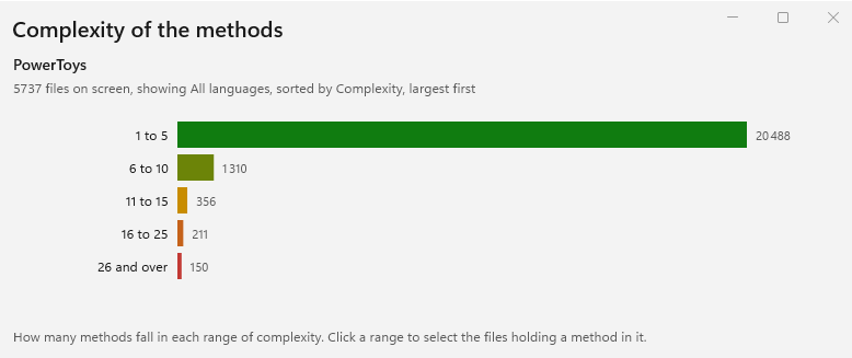
Charts → Complexity histogram counts the methods on screen across ranges of complexity. A healthy codebase is a tall bar on the left and a thin tail. A click on a range selects the files holding a method in it, worst first, which turns "we have complex code somewhere" into a list of files.
Files by complexity
Charts → Files by complexity puts every file on screen as a dot, statements across and complexity up. The cloud shows the relationship between size and difficulty, and the dots that sit away from it are the files worth looking at. Sweep a rectangle over any part of the chart to select the files inside it.
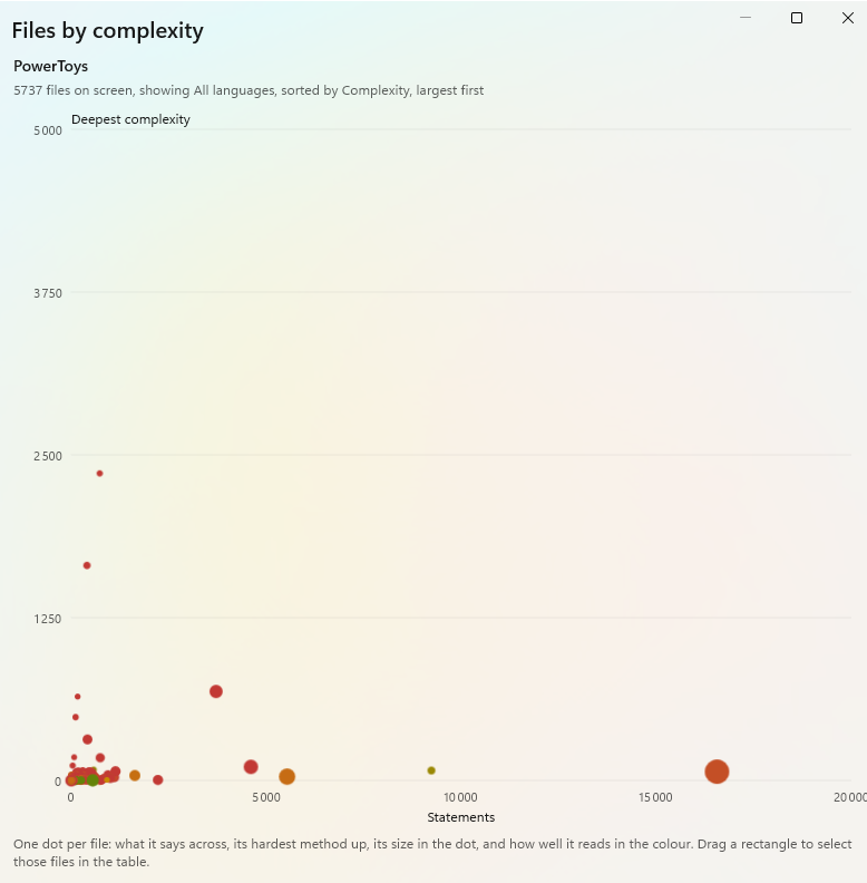
Because a chart can be swept, a click is decided when the pointer comes back up. A press that turned into a rectangle was never a click on whatever happened to be under it.
Language Charts
Two charts say what a codebase is made of, one about the languages it is programmed in and one about the language its people write in.
Languages
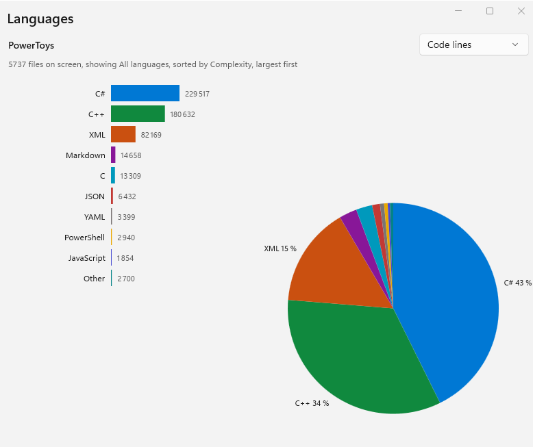
Charts → Languages chart draws the languages of the rows on screen, as bars and as a pie, by files and by lines. The two often disagree, and the disagreement is the interesting part. Clicking a language selects its files.
Human languages
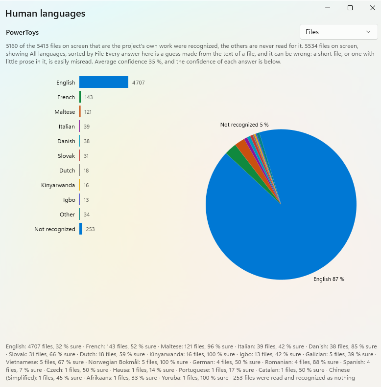
Charts → Human languages draws what the comments and strings are written in, with how sure each answer was. Only the project's own files are counted, since what a generator or a vendor writes its comments in says nothing about the people working here.
Analyses
A run is a throwaway measurement until you keep it. Keeping it gives it a name and writes it into the project, and it becomes a point you can come back to, compare against, and report from.
Keeping a run
The Analyses panel lists what the project has kept, most recent first, with the current run at the top while it is still unkept. Keep… names it and adds it. Closing a project with an unkept run asks whether to keep it or drop it, so nothing is lost by accident.
A name is used once, because a comparison later asks for it by name. Remove drops a kept analysis, or discards the current run when it was never kept. Removing cannot be undone, and what was measured then cannot be measured again.
Looking at an old run
Picking a line of the panel shows that analysis in the table, with its own numbers, its own charts and its own exports, without measuring anything again. The whole window becomes that day's codebase.

An analysis is self-sufficient. It carries the files it measured, the rules it was measured under and the folders it covered, so a project opened years later still explains itself.
Comparing & Trend
Two analyses make a comparison. Three or more make a trend.
Trend across analyses
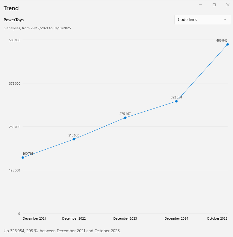
Charts → Trend across analyses draws how one number moved across everything the project has kept, the current run included. Code lines, files, complexity per method, and the rest. The chart says how many analyses it covers and the dates it spans, so a rise is never read as a week when it was a year. The entry stays off until there are two points to draw a line through, the run in hand counting as one of them, and Analysis → Files that could not be read is off in the same way while the last run read everything.
Comparing two
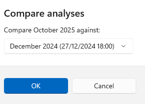
Compare… in the Analyses panel takes the analysis you picked and asks what to compare it against. The result says what moved and which way, in the same words the report uses.
A trend is only as honest as its rules. Because a project freezes its counting rules with its first kept analysis, every point on the line was measured the same way, so a move on the chart is always a move in the code.
Churn from Git
A trend needs analyses you kept. Your repository has been keeping its own account since the first commit, and Code Contour can read it.
A folder inside a git checkout shows a small history mark in the Folders list. When at least one of them does, Charts → Churn from git history opens the chart of what was written into it: lines added above the line, lines removed below it, one column per month.
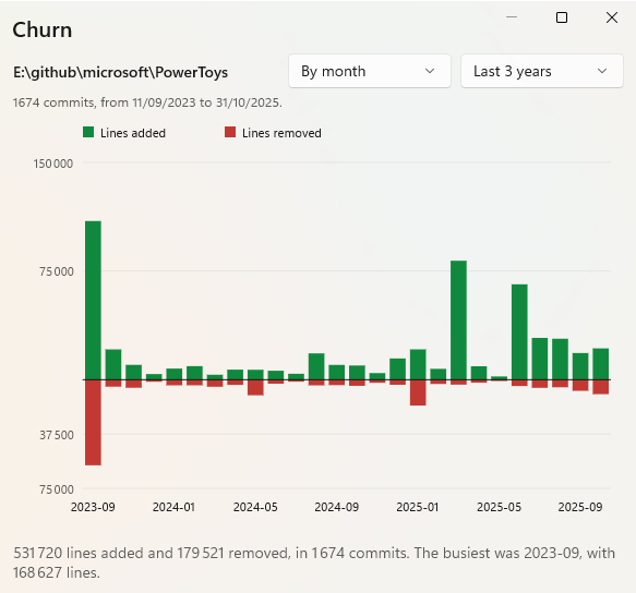
| By month | One column per month between the first commit read and the last, quiet months included, so a year of work is never drawn as though it were busy throughout. |
| By author | The twelve busiest people, largest first, with names resolved through the repository's .mailmap, since the same person often commits under several addresses. |
| How far back | The last 12 months, the last 3 years, or the whole history. A long history takes a few seconds to read, once, and is kept for as long as the window is open. |
| Several repositories | A project whose folders live in more than one checkout adds them up, and each repository is read once however many folders point at it. Two worktrees of one repository are one history, not two. |
| Renames | A moved file is counted as a move, the way git counts it by default. Without that, one afternoon of tidying reads as a heroic week. |
Nothing leaves your computer. The library Code Contour reads repositories with is built without any network transport at all, so it reads the checkout on your machine and cannot contact a server even if asked to.
In the reports
The chart is one window, and the same history goes into the reports when you ask for it. Analysis → Project Settings has Include what the repository was written in reports, offered whenever one of your folders is inside a checkout and explained where none of them is. It belongs to the project rather than to the application, so it travels with the .codecontour file and a build reading that project reports the same thing you do.
| HTML and PDF | A What was written section: the monthly chart, then the busiest people with what each added, removed and committed. |
| JSON | A churn object carrying the repositories, the period, every month and the busiest authors. It is null when no folder is in a repository, which is not the same fact as a repository nobody wrote in. |
| CSV | Nothing. A sheet is one table of files, and churn is a table of something else. |
| How much | The last two years, and the ten busiest people. A report is written while you wait, and a whole history takes far longer to read than a report should. |
| From a script | --churn on analyze and show, or nothing at all when the project you pointed at already asks for it. |
Churn says what was written. It cannot say what was rewritten: only two measured analyses can tell a rewrite from growth, which is what the work report is for. The two answer different questions and are worth reading together.
The Work Report
A trend says where the codebase got to. The work report says what was done to get there, between any two analyses the project kept.
| Written | Lines added that were not there before. |
| Deleted | Lines that went away. |
| Rewritten | Lines written over code that was already there. This is the bar worth looking at, since a codebase being fought with is mostly rework. |
| Touched | Files that changed at all, and the ones that only moved. |
| Which way it went | Whether complexity and maintainability improved or got worse over the period, and in how many files. |
| Where the work went | The files that absorbed the most of it, with the long tail counted rather than listed. |
The period is named at the top, the two analyses and the days between them, because the same amount of work over a week and over a year describes two different codebases.
The report writes as a spreadsheet, a page, a document or a PDF, and the command line writes the same file with its work command.
The detailed work report is part of Code Contour Premium. Without it, Changes since previous analysis gives a real answer in six lines, code lines, files, complexity, maintainability, and which way the methods went.
Exports
Everything on screen leaves the application in the shape you need, and every export covers exactly the rows you narrowed to.
CSV
The table as it stands, columns and all, in the dialect Excel opens as columns on a double click. Ctrl+E.
HTML report
The whole report as one self-contained page, charts included, drawn as vectors so it prints and zooms cleanly. Nothing is fetched from anywhere when it opens.
JSON
The whole analysis as a document with a versioned schema, written field by field so it is a contract rather than an internal type. This is what a build reads.
PDF report
The printed report, see The Report on Paper.
Every report carries the same footer, the product and version that wrote it and the date it was written, so a page found later can always say where it came from. The HTML, PDF and JSON reports also carry what the repository was written when the project asks for it.
The HTML report's file names are links. Clicking one opens that file in Code Contour, at the line, through the codecontour: link the application registers. A report you send to somebody who has the tool is a report they can walk into.
The Report on Paper
File → Export report as PDF writes the report as a real printed document, with no browser anywhere in it.
It says the same things the window says, in the same words, and leaves out what only a screen can carry. Every file of a run would be a hundred pages of paper and a scroll bar on a page, so what is printed is the summary, the charts, the rankings and what is worth looking at.
The pages are laid out the way a document should be. A heading is never left alone at the foot of a page, a table that does not fit is split and writes its headings again at the top of the next page, and a path in a cell is shortened in the middle so the file name always survives. Page size follows your region, A4 or Letter.
The charts in the PDF are the same charts the windows draw. The arithmetic is written once, so a chart on screen and a chart in a report can never disagree about where a point sits.
Command Line
Code Contour carries a console application, so a build can measure what a developer measures, under the same rules, and stop when a limit is passed.
Getting it
File → Extract the command line tool writes the executable wherever you ask. It is one file, with no runtime beside it, which is what a build agent wants to unpack. The copy it writes names the person it was written for, so a copy that turns up elsewhere still says where it came from.
Commands
| analyze | Measures folders, or a project, and writes what was asked for. |
| show | Reads an analysis a project kept and writes it, without measuring anything again. |
| analyses | Lists the analyses a project kept, and removes one when asked. |
| work | Measures the work done between two analyses a project kept. |
| churn | Reads what was written into the repository a folder is in, by month or by author, without measuring anything. |
| --churn | A switch rather than a command: analyze and show put the churn into the HTML, PDF and JSON reports they write. |
| languages | Lists the languages this tool reads, by identifier. |
| extensions | Lists every extension it has an opinion about, and what was decided for it. |
| info | Says what this is and what it is running on. |
| license | Says who this copy was written for. |
Each of the four operational commands writes any of the four shapes, --json, --csv, --html and --pdf, and --json - writes the document to standard output so a pipeline can read it. --project reads a project saved by the window, so a build measures what the developer measures. --keep writes the run into the project, which is how a build gets a history of its own.
Exit codes
--max-complexity and --min-maintainability are the limits, and a limit nobody gave is a limit nothing can fail, so a run with neither only reports. What failed is said on standard error, which leaves standard output to whatever was asked for.
The extension mapping is looked for in three places, in the order you would expect: the file named by --settings, then a settings file sitting beside the executable, which is how a copy dropped on a build agent carries its own rules without touching that machine's, then the settings the application writes for the person logged in.
Settings
Settings belong to you and follow you between projects. Rules that decide how a number is counted belong to the project instead, so a history is never measured two ways.
| Appearance & behavior | Theme, and how the window behaves. |
| File extensions | What each extension is, and which ones hold no code. |
| Human languages | Which human languages you expect to meet in code. A file is shown as the first language of its list that you expect, and one whose whole list is unexpected is flagged for you to look at. |
| What counts as normal | The band each metric is compared against, which is what the Kiviat draws. |
| Remember reading | Whether the place you left a file at is kept, so it opens there again. |
| Projects | Recent projects, and what a new project starts with, including whether it leaves code that is not your team's own work out of the analysis. That one is off to begin with, since measuring it and marking it in its own column is what keeps the totals honest, and each project can decide for itself in Analysis → Project Settings. |
| Storage | Where the settings live, with a way to open the folder. |
Any file can be read in any encoding Windows knows. A project says which encoding a file with no byte order mark is read in, and the list puts the ones a codebase actually meets first.
Keyboard Shortcuts
Project
Analysis
Charts & viewer
Tips & Tricks
Start with the map, not the table
Open Map of the code and colour it by Outside. Before any metric means anything, you want to know how much of what you just measured your team actually wrote.
Turn a worry into a list
"We have some complex code" is not actionable. Open the Complexity histogram, click the worst range, and the table becomes the list of files to look at, worst first.
Keep a baseline on day one
Keep an analysis before you start work on a codebase, and name it for the date. Everything you do afterwards is measurable against it, and the work report can tell you what a month of effort actually changed.
Exclude once, not every time
Exclusions and the inside or outside answer you give a file are remembered with the project, so a tree full of vendored code only has to be sorted out once.
Put it in the build
Write the command line tool out, drop it on the agent with a settings file beside it, and run analyze --project with --max-complexity. The build fails with exit code 2 the day something crosses the line, and --keep gives the build a history of its own.
Send the HTML, not a screenshot
The HTML report is one self-contained file with the charts inside it, and the file names in it are links back into Code Contour. It is the fastest way to hand a codebase review to somebody else.
A quick rating on the Microsoft Store is the best way to say thanks. It helps other developers find Code Contour, and it takes less than a minute.
★ Rate Code Contour on the Microsoft Store